The Development of Collective Structure and its Response to
Environmental Change
Norman L. Johnson
Theoretical Division
Los Alamos National Laboratory
MB B216, Los Alamos, New Mexico USA
nlj@lanl.gov
ABSTRACT
How do collective processes in decentralized,
self-organizing systems respond to environmental change? What are the
contrasting roles of collective structures and innovative components
(variation, diversity, entropy), and how do these roles change with different
rates of environmental change? To answer these questions, a simple
self-organizing system is examined – a simulation of foraging for food by ants
in the presence of environmental change. This model system has been argued to
be similar in dynamics to decentralized components of many collective systems -
ecologies, economies, knowledge systems, societies, political systems, etc. The
simulations are first shown to illustrate a developmental view of evolving
systems, captured by the developmental stages of Formative, Co-Operational and
Condensed. The effects of different rates of environmental change are then
presented. For small rates of change, the system productivity is largely
unchanged. As the rate increases, innovative information becomes more important
to sustaining the productivity. As the rate further increases, episodic failure
is observed as stabilizing collective structures fail, and the system regresses
to earlier developmental stages. The collective structures are shown to inhibit
the performance of the system as a whole in rapidly changing environments. A
quantitative measure is developed that captures the efficacy of the collective
structure. A variation of the system with a mechanism for sustaining collective
structures is found to be more sensitive to environmental change, duplicating
the decline in productivity observed in aging systems.
1
INTRODUCTION
The following study begins with the assumption that
decentralized, self-organizing processes are key components to many systems and
then focuses on what insights can be gained about the nature of these processes
in a specific model system in the presence of different rates of environmental
change. “Environmental change” is used to describe aspects of a system (e.g.,
boundary conditions or coupled systems) that are typically assumed constant or
slowly changing. The understanding that environmental stability is required for
the development of ecological systems has been present since early studies (Conrad
1983), but a general understanding of the dynamics across the different stages,
with and without environmental change, appears to be missing. The relevance of
such an investigation is becoming more apparent in a world has fewer components
that are in
stasis.
The object of this study is an agent simulation of
an ant foraging system, which has been extensively studied both in nature and
computationally (Bonabeau et al 1999). This system represents the popular
example of an “organism” (system of processes) that has no centralized
coordination of its components (agents), where the capability of the components
are simple compared to the capabilities of the “organism” as a whole, and where
the fundamental processes (reinforcement of individual pheromone trails) have
been used to solve a variety of challenging problems (Bonabeau et al 1999).
2
MODEL DESCRIPTION
The agent simulation tool chosen is StarLogo, a
cross-platform, public-domain software that is maintained by M.I.T’s MediaLab
and available at their web site.
This software was selected over others because of its simplicity to use and
modify, because of its availability to enable experimentation beyond the
studies here, and because it provides a documented example of ant foraging.
The example ant-foraging problem in StarLogo is
defined as follows (see Figure 1). One hundred ants using identical rules
forage on a periodic square domain (e.g., if an ant leaves the top, it reenters
the bottom). The domain is discretized into 101 divisions in the two
dimensions. The agents have only three rules of action: 1) if food is found,
pick it up and return to the nest, leaving an evaporating pheromone trail
behind, 2) if an agent has food and is at the nest, then drop the food and
reverse direction 180 degrees and search for food, 3) when searching for
food, follow the shared information (pheromones) to the source, otherwise
search randomly. In the two operations of returning to the nest by the radial
pheromone field (see Figure 1) and by following the shared information to the
source, an estimate of the gradient of the “information” field is made and the
agent attempts to follow the increasing gradient. Note that the radial field
for returning to the nest approximates a globally aware mechanism for returning
to the nest (Wohlgemuth, et al 2001). The agents move one space per time step
(or time unit), so in 50 time units
an agent can move from the nest to the closest periodic boundary in a direct
line.
While the above model is unsophisticated by
comparison to scientific models (Bonabeau et al 1999), it does capture the
essential features of foraging behavior: of exploiting the closest sources
first, of requiring additional resources to optimally exploit food sources far
from the nest (longer trails require more reinforcement), and of exploiting one
food source at a time when two sources are equidistant. By expressing a variety
of realistic behavior, the example simulation is a reasonable choice for the
present study. While not examined, likely other implementations would duplicate
the same conclusions as the present study.
The example allows the user to modify the evaporation rate and the diffusion rate of the pheromones in
order to examine the effect of these parameters on the performance of the
system. The diffusion mimics the spatial diffusion by Fick’s Law: at each time
step a percentage of the pheromone in a storage location will be transferred to
its eight neighboring locations. For example, if the diffusion rate is set to 12%, then 0.12 of the pheromone will be
transferred (0.015 of the pheromone to each of the eight neighboring
locations). The evaporation is the reduction at each time step of the
pheromones in the entire domain by a percentage set by the evaporation rate. For example, if the evaporation rate is set to
4%, the pheromone level at each storage location will be reduced by 0.04 of its
value at each time step. Therefore, an evaporation rate of 100% removes all
pheromones at each time increment.
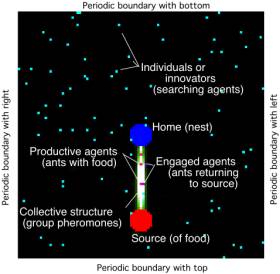
Figure 1: Identification of the components of the simulation. Not shown is
the permanent pheromone field that is created at initialization that enables
the agent to return to the nest; it decreases radially from the nest to the
boundaries.
The original example is modified in one way (aside
from a variety of diagnostic additions described shortly) and the setup file is
available at the author’s website.
The original movement of the agent in the domain was more random and was set to
vary at each step by an increment of plus or minus 40 degrees from its current
direction (sampled from a uniform distribution). In the following simulations
this variation is reduced to plus or minus 10 degrees for random foraging and
plus or minus 5 degrees for returning to the nest. These changes tend to cause
less randomness in the individual movement from a straight line, but no
qualitative differences are observed in the results reported below, and
quantitative differences are within the variations from run-to-run of the
simulations examined. The values for all following simulations (except where
noted) use the evaporation and diffusion rates of 4% and 12%, respectively.
Finally, the setup (initial) conditions of the
original example are modified. Instead of three stationary food sources of a
limited supply (given sufficient time, each source will be used up), one
stationary (or moving) source of unlimited supply is created in the domain.
When stationary, the unlimited nature of the supply enables the exploitation of
the source to reach steady state (to within the natural variation of the
system).
To enable the foraging simulations to have broader
applicability, the following nomenclature is used and subsequent diagnostics
are based on these definitions (see Figure 1). The agents (models of ants) leave information (pheromones) on the
domain when they are returning to the nest with food. If the pheromone cloud
persists on the domain as reinforced by the combined pheromones of the agents,
it is called a collective structure.
Note that for the distance of the source and the evaporation and diffusion
rates chosen, a single agent cannot sustain a collective structure. A collective is a group of agents that
have gotten food and are still within the collective structure. Agents in the
collective are either carrying food to the nest or do not have food but by
design, they are following the maximum gradient of shared information (pheromones)
that might lead to a source. Agents
that are not part of the collective are individuals
(also called innovators, when the individuals
play an essential role). Note that an individual can either be outside the collective
structure and randomly searching or can be within the collective structure but
not have found the source yet. The above concepts of a collective and
individuals are only for the purposes of analysis and do not affect the
simulation in any way.
The productivity of the system as a whole is
defined as the rate that the source is exploited. Similarly, the productivity
of the collective and individuals are the rates that the collective and
individuals exploit the source, respectively. The productivity is defined as
the rate of food taken from the source. (An alternative definition of
productivity is based on the deposition of food at the nest, but it is not used
in order to avoid the intrinsic time delay in this measure, caused by the
transit time of the agents returning to the nest.)
3
STAGES OF DEVELOPMENT
To aid in the analysis of the effect of environmental
change, the following view of the developmental
stages of self-organizing systems is introduced for stable environments and
is discussed in detail elsewhere (Johnson 2000; Johnson 2002). This perspective
is closely related to the developmental theory proposed by Salthe for
biological (ecosystems, etc.)(Salthe 1989; Salthe 1993a; Salthe 1999)
and sociological systems (society, economies, organizations) (Salthe 1993b). To
date, the primary difference between the two developmental views is that
Salthe’s focuses on the interplay of developing structure and free
energy/information (entropy) of system as the system maturates and declines.
This is contrasted to the current perspective that focuses on the processes of
system optimization at different stages of development. The current study
offers new insight as to the connection between the two theories and is
discussed in section 5.
Because “structure” is a core concept to the
developmental cycle, clarification is needed as to what is meant by it (for a
complete discussion see (Johnson 2002) and (Bedau et al 1998)). In the above
introduction, structure is used to describe sustained features of a system that
direct the evolution of the system, as might be captured by genetic adaptations
or social institutions. In the analysis herein, “structure” is used to describe
the collective pheromone paths, which require reinforcement to be sustained.
Both usages of “structure” convey how evolved features affect the future
dynamics of the system by limiting the exploration of the potential options of
the system. The difference between the two types of structure, internally
versus collectively sustained, is important when environmental change is
considered (discussed in section 5). In the following discussion, they are
considered equivalent.
Figure 2 summarizes the three stages, as they would
apply to the current system. There are many ways that the developmental process
can be viewed: 1) the origins of system-wide function or performance, 2)
the roles of diversity in the dynamics of the system or 3) the chaotic nature
(or not) at the local and global levels of the system. Each of these
represents different perspectives of the same underlying processes, but they
are often treated separately in the absence of a unifying viewpoint. Each of
these viewpoints is discussed in turn.
3.1
THE ORIGINS OF SYSTEM PERFORMANCE
The system performance, in this case defined to be the
rate of production, is initially from individuals that happen to randomly
locate the source. The random discovery of the source is the most decentralized
(uncoordinated) stage of the system and illustrates the initial vague or completely
undefined state of the system.
Because the agents do not
genetically evolve or remember complex past states or have finite lifetimes,
the formation of individual definition (features
or capabilities of agents) by selective processes (i.e., natural selection) in
the Formative stage (Johnson 2002) is
not as richly expressed in this example as in other systems. In the current
system, the creation of definition is
limited to individuals using their limited memory of what direction they are
going to optimize there own food gathering. For example, because the agents in
the current simulations reverse their direction after leaving food at the nest,
during the initial exploration of the system the population becomes more
“defined” as individuals are “self-selected” to concentrate on the sector where
the source resides. This self-selection of direction is independent of the
effect of the pheromones trails and causes an improvement in the production
rate in the Formative stage, above the simple random discovery of the source.
This increased production can be observed by comparing two simulations with a
high evaporation rate (i.e., no collective effects are possible): one
simulation with a 180 degree reversal in direction after depositing food at the
nest and the other with a random selection of direction after depositing food;
the simulation with the 180 degree reversal shows the higher productivity
associated with the Formative stage.
The further development of the system beyond the
Formative state depends on the details of the specific simulation. For example,
if the population is sufficiently dispersed (low spatial density) or the source
sufficiently distant, the individual pheromone trails are not sustained for
collective use and only independent individuals contribute to the productivity
(as in the first graphic in Figure 2). Under these conditions, the system will
remain in the Formative stage.
If there is a sufficient spatial concentration of
agents and the source is sufficiently near to the nest, the individual pheromone
trails will begin to self-assemble, creating a collective structure. This is the beginning of the Co-Operational stage. The choice of
“Co-Operational” is meant to capture the processes by which agents solving
individual problems, primarily on their own, but on a common problem domain,
contribute to higher collective performance (Johnson, 2000). The Co-Operational
stage is the transition between the system productivity dominated by individual
performance to being dominated by collective performance. For the current
simulations, the higher performance in the Co-Operational stage is the
increased efficiency of food collection when the individuals use the collective
structure to optimally locate the source, rather than using a random search.
This collective assistance occurs either when agents within the collective drop
off food at the nest and are then guided to the source or when individuals
randomly encounter the collective structure and then are guided to the source.
The higher performance by the collective in the
Co-Operational stage can also be expressed as the collective “discovery” of the
shortest path between the source and the nest and as the exploitation of the
food sources that are closest to the nest. Both of these lead to higher rates
of productivity and are the expression of emergent
properties of the system – a global property that cannot be determined from
knowing the properties of the individuals alone. Note that in the
Co-Operational stage, there is productivity both from the collective agents and
from the individuals. In the Condensed
stage, most of the agents are part of the collective, and the system performance
is maximized and resides primarily in the collective production. Figure 3
quantifies the above observations for the simulation illustrated in Figure 2.
Note that because of the random nature of the simulations, identical results to
Figures 2 or 3 may not be duplicated, but averaged quantities should be
similar.
The upper
graphic in Figure 3 shows the total food production of the system. Note the
intervals between 100–150, 150–400, and 500–1000 time units have approximately
constant slopes with values of 0.14, 0.43, 1.01 food units/time unit. These
correspond to the three stages described above. (The slope in the Formative
stage is extremely variable and the value given above is for a run with a high
rate of evaporation, which prevents the transition to the Co-Operational stage
and yields a reproducible value.)
The increased production in each subsequent stage corresponds to
the increased influence of the collective structure, as noted above. Because of
the chaotic nature of the agents, the regions of transition between the stages
will vary from run to run. For example, a run using different seeds for the
random number generators (which determine random choices of direction for the
agents) result in different curves and different transitions for the three
stages. Because the environment is fixed in this simulation and because of the
parameter choices for the evaporation and diffusion rate, there is a strong
drive for the system to develop to the Condensed state, and no variations from
run-to-run were observed to prevent the system from achieving the Condensed
state. As noted earlier, operating parameters and initial conditions can be
chosen (e.g., the evaporation rate or the source location) which can shift the
transition regions or stall the developmental process entirely, even for a
constant environment.
Figure 3:
Plots of various measures versus time in the approach to steady state by the
system. “Collective” refers to the agents that are actively engaged in
production within the collective pheromone structure (see text). “Individuals”
refer to the agents that are not part of the collective. The “collective age”
is the average time that an agent in the collective is continuously productive.
The “structural efficiency” is a measure of the efficiency of the collective
structure; a negative value means the collective structure is inhibiting the
global system performance.
All the measures in Figure 3, except the plot of the
total food, require the definition of a collective defined in section 2 (agents
that have found food and thereafter are continuously in the collective
structure). Being “in” the collective structure is defined as being within a
sustained pheromone strength greater than 0.05 concentration units (similar to
the extent of the pheromone clouds plotted in Figures 1 and 2). Any agents not
in the collective are individuals or innovators. Note that an individual can be
in the collective structure, but not part of the collective until it finds the
source. Hence, this definition of collective is based on productivity, not just
the sharing of information. An alternative definition, and possibly more
commonly made, is based on agents within the collective structure. Within a
stable environment, both of these measures would yield similar results, but in
a changing environment, the definition herein focuses on the critical aspect of
the system, the productivity.
Given this definition of the
collective, a variety of measures can be defined, as illustrated in Figure 3.
For example, the number of agents in the collective can be divided by the total
population (100) —this is plotted as the fraction
of the population in the collective. Similarly, the rate of production (of
food) by the agents in the collective can be divided by the total rate of
production — this is the fraction of
production by the collective. (Note that the fraction of production by the
individuals not in the collective is just unity minus the fraction of
production by the collective.) Another useful measure is based on the duration
that an agent spends continuously in a collective. The average of this duration
or “age” of the collective is plotted as the Collective age. Note that the collective age does not continually
increase in the Condensed stage, because of the failure of the agents to stay
in the collective structure due to errors in tracking the pheromone gradient.
Hence, even in a stable Condensed stage, one third of the agents on average are
outside of the collective.
The final collective measure, the structural efficiency, is a direct
measure of the efficacy of the collective structure in the system productivity.
The structural efficiency is found from the difference between the fraction of
food collected by the collective and the fraction of the population that is in
the collective (the difference of the two upper curves in the bottom graphic in
Figure 3). It is bounded between unity and minus the faction of the population
in the collective.
A more intuitive, but equivalent, way to define the
structural efficiency is as the difference of two production rates (and then
divided by a total production rate to make it dimensionless): the actual rate
of production from the collective minus the rate of production from the
collective if the collective effect was neutral (i.e., production just by
numbers). Hence, the measure represents the additional efficiency of the
collective. By multiplying the structural efficiency by the total production
rate, the added production rate of the collective can be found. The creation of
a measure that focuses on the effect beyond a neutral process parallels the
approach taken by Bedau in defining lasting adaptations beyond neutral
adaptations (Bedau et al 1998).
For example, if the structural efficiency is zero,
then the production by the collective and individuals are proportional to their
relative numbers. If the collective production is higher than predicted from
its proportional representation, then the structural efficiency is positive. If
the production by the individuals is relatively higher, then the structural efficiency
is negative. Because the structural efficiency is calculated from the
difference of two noisy, largely uncorrelated numbers, it exhibits large
fluctuations as observed in Figure 3 (for a longer average from 1000 to 5000
time units, the structural efficiency for the base simulation is 0.14 with a
standard deviation of 0.08). Note that the decline in the structural efficiency
in Figure 3 is anomalous to this run.
3.2
ROLES OF DIVERSITY IN THE SYSTEM
Many different measures can be defined for diversity in a
decentralized agent system, from local to global measures (see (Johnson 2000
and 2002) for a more complete analysis of the different types of diversity and
their influence on self-organization). In the current simulations, all of the agents
have the identical rule set (the three rules listed in section 2) and minimal
memory (the current direction of movement and “do I have food or not?”), so
local diversity measures that are based on agent differences are limited and
are largely captured by the distinction between the collective and individual.
A more useful measure is the global or domain
diversity, captured by the spatial
location of the agents in general, and by the sector location in specific. It
is easy to see how this domain diversity might become important if the sources
were randomly placed in the domain as a variation of the current simulation. An
agent population with low domain diversity will be slow to discover the new
sources. The correlation between discovery and domain diversity is a feature of
the Formative stage, similar to the arguments used for selection from genetic
diversity in genetic algorithms (Fogel 1999).
The selection from a variety of individual
“discoveries” is part of the process of creating definition in the system, as described
in the previous subsection. In the current simulation, the agents increase
their definition by reversing their direction after dropping off food. This
increased definition of the agents reduces domain diversity, but also increases
the likelihood of the Co-Operational stage to form, by increasing the density
of agents in the vicinity of the source. The general observation is that for
the global system to improve its performance in the Formative stage – as based
on the average individual performance, diversity is consumed. At any time in
the process of selection, if diversity is not consumed or is regenerated, such
as using a random selection of directions after dropping off food, then the
system performance will be degraded by the presence of individual performers
with lower productivity.
In the Co-Operational stage, just the opposite
dependency on diversity is generally observed: diversity is required for the current system performance, and not as
an investment for future system performance as in the Formative stage. For example,
in the emergent discovery of a shorter path to a source (emergent because no
individual has a global perspective), it is the combination of many diverse
paths that leads to the shortest path (Johnson 2000), not the selection of one
optimal path of a single individual from a diversity of paths. For this synergy
of diverse individual contributions to be optimally expressed, the domain must
have features that limit options beyond those that exist in the present simulations.
One way to introduce such features is to put obstacles in the domain. Because
other studies (Johnson 2000; Johnson 2002) focus on this feature of the
Co-Operational stage and because the emphasis here is on the simplest model for
studying environmental change, the added complication associated with a rich
expression of this feature is not introduced.
In the Condensed stage, the
collective structure strongly reduces the domain diversity of the population,
as illustrated in Figure 2 — most of the agents are located in one sector of
the system. The strong coherence, and hence the low diversity of the agents, is
the signature of the Condensed stage.
In summary, for the current
simulation with a fixed source of infinite supply, the domain diversity is reduced
in the Formative stage, relatively unchanged in the Co-Operational stage, and
is low for the Condensed stage. The changes of the system productivity
presented in the last section can be viewed from the perspective of the
interaction of the domain diversity in the system with different processes in
each stage: the process of selection from diversity in the Formative stage, the
synergistic combination of diversity in the Co-Operational stage, and the
optimization in the Condensed stage.
3.3
THE LOCAL AND GLOBAL CHAOTIC NATURE
One of the more illuminating views is the degree of
randomness or predictability exhibited by different levels (local or global) of
the system in the different stages. The initial vague state where the
production is from random discovery of the source is the most chaotic state,
both in the movements of the agents (local) and in the system productivity
(global).
The Formative and Co-Operational stages when viewed
locally at the agent level, both have a significant chaotic nature, expressed
by the individuals that are not part of the collective and expressed by the
increased chaotic movement of agents during the formation of the collective
structure (this can be demonstrated by reducing the sensitivity of the agents
to the pheromones or reducing the total number of agent, both which prohibit
the Condensed stage from forming).
In the Condensed stage, most
of the agents are captured by the collective structure and are therefore
predictable. While not quantified, these observations can be made from an
animation of the spatial placement of the agents, as in Figure 2. The
difference in coherence in the collective structure between the Co-Operational
stage and Condensed stage is captured quantitatively by the change in the
collective age in Figure 3. While not shown, the standard deviation around the
mean collective age is much greater for the Co-Operational stage than for the
Condensed stage.
From a system or global view of production, the
Formative stage is highly irregular - dependent on the random actions of
uncoordinated individuals. But the productivity in the Co-Operational and
Condensed stages is predictable (illustrated by the fixed slope of the total
food curve in Figure 3), because of the stabilizing effect of the collective
structure in a stable environment.
This leads to the observation that the developmental cycle can be viewed as an
interplay between evolving structure and randomness around this structure. This
is also argued by Salthe in his developmental theory (Salthe 1993a).
In this section, the development of a simulation of
foraging through progressive stages is examined for a stable environment from
three viewpoints: the processes of productivity, the changes in diversity and
the degree of chaotic behavior at local and global levels. The developmental
perspective unifies these three viewpoints, describing how different processes,
each with different degrees of chaotic behavior at the local and global levels,
can operate on different degrees of diversity to yield various rates of
productivity.
4
EFFECT OF ENVIRONMENTAL CHANGE
Given the above characterization of the model system in a
stable environment, the effect of a changing environment on the system is now
examined. The integration of these results with the developmental perspective
is presented in section 5.
There are many ways that the system described in
Figure 1 can be modified to capture the idea of environmental change. The one
chosen is illustrated in Figure 4, in which the source is moved in a circle of
constant radius at a fixed angular velocity from the beginning of the simulation
(i.e., there is no establishment of a stationary state before rotation begins).
By imposing different angular velocities, different rates of environmental
change can be examined.
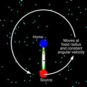
Figure 4:
Implementation of the environmental change. The unlimited source from Figure 1
is moved in a circle with a fixed angular velocity. Note that no food is left
behind as the source moves.
The simplicity of the presentation of this
implementation and its ease in testing in an actual foraging experiment are the
main reasons for its choice over alternatives. In fact, different alternatives
were tried (such as gradually increasing the rotation rate of the source,
starting and stopping the source, or making the source travel on an ellipse
instead of a circle), but the choice in Figure 4 expressed most of the observed
results.
4.1
CHANGES IN PRODUCTIVITY
The rates of production for the
different angular velocities (rate of
environmental change) are shown in Figure 5, along with a breakdown between
the collective and individual contributions and with the standard deviation of
the total production of the underlying data. Note that the results are reported
for the time interval from 1000–5000 time units, after the initial transients
have passed. These results represent a stationary state of the simulations, but
not necessarily steady state behavior (i.e., the system may exhibit repeated
transient processes that prohibit the approach to a fixed steady state).
To give some perspective of the magnitude of the
rates used, at a value of 0.8 degrees/time unit (8 on the figure), the source
at the specified radius moves at about half the speed as an agent traveling in
a straight line (1 step/time unit).
Three major observations are made based on Figure 5:
·
The system productivity drops as the
rate of environmental change increases.
·
The decline in the contribution from
the collective is the major cause of the drop in
production.
·
The variation (standard deviation) in
the productivity increases significantly between 0.1 and 0.3 degree/time unit,
suggesting a change of stability in the simulations.
|
|
|
Figure 5:
Rate of production for different rates of environmental change from an
average over 1000-5000 time units, broken down into contributions from the
collective and individuals. The bars represent two standard deviations from
top to bottom of the underlying data.
|
The animations for the simulations
that are the basis of the results in Figure 5 provide an understanding for
above observations. As the environmental rate increases, the following progression
is observed:
·
For the environmental rates from 0.0
to 0.1 degree/time unit, there is little change in the dynamics or productivity
– the collective structure forms and exhibits no significant difficultly
adjusting spatially to the moving source.
·
For the environmental rates from 0.1
to 0.2 degree/time unit, while the system as a whole retains most of its
productivity, the individuals or innovators
become essential for sustaining the collective structure in the region of the
moving source. The reoccurring pattern is that the collective can quickly
exploit the new location of the source in great numbers once an “innovator”
finds the new location. The collective
never contributes to finding the new location of the source. The pheromone
trail of the innovator is the only connection between the misplaced swarm and
the new location of the source.
·
At the environmental rate around 0.3
degree/time unit, the system expresses boom-and-bust cycles (so named because
of the resemblance to stock market cycles). The collective structure
experiences periodic collapse when it cannot continually track the moving
source, and consequently the production rate has a much greater standard deviation.
·
At the environmental rates beyond 0.3
degree/time unit, the collective structures that continually form are not
located near the current source; hence, the exploitation of the collective
structure rarely occurs.
Note that the above observations at the extremes of
environmental change (small and large) are not path dependent – simulations
that let the system come to a “steady” state (the Condensed stage) before the
source is moved result in production rates similar to those in Figure 5.
For three of the rates of environmental change (0,
0.2, 0.8 degree/time unit), the transient values of the production rate are
presented in Figure 6. (The averaged values in Figure 5 are for the time
interval from 1000-5000 time units of this figure. Note that the cumulative
integral of the “rate = 0” curve over time is the total food curve in Figure
3.) Note that the two extreme values of the environmental change exhibit less
fluctuation, compared to the intermediate value of 0.2 degree/time unit. The
intermediate rate is rarely as productive as the simulations with a stable
environment, but neither does it degrade to the low productivity of the
simulations for the most rapidly changing environment. It does exhibit one
“bust” at a time of 1000 time units. For the rate of 0.1 degrees/time unit, the
system never was observed to exhibit a total collapse of the collective
structure.
4.2
THE “BOOM-AND-BUST” TRANSITION
One of the detrimental aspects of the real world
boom-and-bust cycle is not only the lower productivity, but also the loss of
resources during the bust phase – if the same (or even reduced) productivity
can be achieved without the “bust,” many of our systems would likely fair
better. Although the resemblance of the current simulations to, say, the stock
market is limited, there may be insights into the processes surrounding the
boom-and-bust cycles in the current system that are applicable elsewhere –
particularly in the role of the collective structure.
Figure 6:
Time-resolved rate of production for three different rates of environmental
change (the rates have units of degree/time unit).
Plotted in a separate figure (Figure 7), but with
the same coordinate ranges at Figure 6, are the time-resolved production rates
for the rate of environmental change that exhibits the greatest fluctuations
(0.3 degree/time unit) – the system that is continually in a boom and bust
cycle. This suggests the following study to better understand the source of the
boom-and-bust behavior.
If the simulation represented in Figure 7 is redone
with double the evaporation rate (8% instead of 4%), the number of “bust”
events are reduced by a third (defined to be the number of excursions of the
production rate below 0.2 food unit/time unit) and the total production is 20%
higher. Effectively the higher evaporation rate reduces the fraction of the
population in the collective structure by 20% overall, thereby freeing up
innovators that can keep the collective structure from collapsing. Hence, the
overall efficiency is increased even though it results in having fewer agents
in the collective structure, because of the importance of finding the new
location of the source. This implies that in times of change it is essential to
allocate properly resources between the collective structure and innovators –
with a greater emphasis on innovation with larger rates of change. As noted
above, this is particularly true if the system of interest has disadvantages
associated with bust phases, such as the loss of resources.
Figure
7: Time-resolved rate of production for the rate of
environmental change of 0.3 degree/time unit.
As
observed earlier for the unchanging environment, there is a positive feedback
process by which a successful collective structure enlists individuals, due to
the strength and extent of the collective structure. In the transient process
of a boom-and-bust cycle, it is observed to be a trend (but not always) that
the bust is preceded by a higher fraction of the production coming from the
collective. This suggests that the bust is indeed proceeded by a “boom,” which
thereby captures resources (innovators) that are needed to prevent a subsequent
bust. The bust then frees up these resources and the new location of the source
is found and tracked by the additional innovators. The new source is then exploited
by the collective, and a boom begins. The success of this boom then repeats the
cycle.
The above interpretation is also supported by the
path dependence of the system for intermediate rates of environmental change.
If the movement of the source is started after the system has fully developed
the Condensed state, it is observed that the inevitable “bust” is more likely
to occur sooner, and be deeper and longer. This observation supports the
hypothesis that the higher coherence of the collective structure is the
possible cause of the subsequent ”bust”.
For completeness is should be noted that this
positive feedback loop in the boom-and-bust cycle is dependent on a fixed
number of agents, which then must be allocated between two essential tasks
(exploitation and innovation). The balance between exploitation and innovation
has also been argued to occur for genetic algorithms (Goldberg 1998). In the
current simulations, if unlimited resources, or at least additional resources
were available, then the boom-and-bust cycle may not occur.
4.3
COLLECTIVE EFFICIENCY (AND INEFFICIENCY) UNDER ENVIRONMENTAL
CHANGE
In the analysis of the system in a constant environment,
the collective was found to increase the productivity. Given a changing environment,
the question arises if this increased efficiency is retained or negated, or is
there in fact an inefficiency associated with the collective structure?
The quantitative measure of the structural
efficiency was introduced in §3 and was defined to be the difference of two
fractions: the fraction of productivity provided by the collective and the
fraction of the population in the collective. In Figs. 8 and 9 the changes of
these fractions are present for the different rates of environmental change. A comparison
of the two figures show that for low rates of change, two-thirds of the
population in the collective (Figure 8) are providing over 80% of the total
productivity. This increased efficiency of the collective declines in the
transitional region of the boom-and-bust cycle, until the collectives are
actually producing less than their proportionate representation.
These observations can be captured in plot of the
structural efficiency (Figure 10), which dramatically illustrates the change in
efficacy of the collective structure. At low rates of environmental change, the
increased efficiency of the collective structure is at its maximum. It then
declines and becomes negative as the collective ties up resources that are best
utilized as innovators. To quantify this inefficiency, a simulation was done
with a high evaporation rate (75%), which inhibited the formation of the
collective, for a rate of environmental change of 0.8 degree/time unit and then
compared to the simulation with the collective forming. The total production
was found to be degraded by 50% in the simulation with the collective
structure. This strongly illustrates that the collective structure is a major
source of inefficiency for the system as a whole when the environment changes
quickly.

Figure 8: The fraction of the population in the collective for different
rates of environmental change from an average over 1000-5000 time units. The
bars represent two standard deviations from top to bottom of the underlying
data.
Figure 9: The fraction of production from collective for different rates of
environmental change from an average over 1000-5000 time units. The bars
represent two standard deviations from top to bottom of the underlying data.
Figure 10:
The structural efficiency (positive when the collective structure increases the
system productivity) for different rates of environmental change from an
average over 1000-5000 time units. The bars represent two standard deviations
from top to bottom of the underlying data.
Figure 10 also shows the sensitivity of the standard
deviation of the structural efficiency in the transitional region, more so than
any other variable previously examined. This sensitivity is amplified by
plotting the coefficient of variability (Figure 11) for the values in Figure
10. This plot dramatically indicates the extreme instabilities and changing
processes in the transitional region. The coefficient of variability is
normally a general indicator of population variability and is measure of
potential that selective processes can operate on a population. The
interpretation here is that the collective structure of system is expressing
the maximum variation (from the extremes of Formative to Condensed) and the
system is in an optimal state to select from this “population.” This suggests
that if the environmental rate quickly increased or decreased in this region of
maximum variation, the system would quickly select the optimal state for the
new rate.
Figure 11: The coefficient of variability (ratio of the mean to standard
deviation) of the structural efficiency for the data in Figure 10.
Figure 12 is a comparison of the time-resolved
structural efficiency for the two extreme rates of environmental change (0.0
and 0.8 degree/time unit) and the transitional environmental rate (0.3
degree/time unit). Not only does the time-resolved structural efficiency
illustrate the boom and bust cycle in the transitional region, it also momentarily
exceeds the values of the collective performance and failure of the system in
the stable and rapidly changing environments, respectively. This supports the
conclusion that the boom-and-bust state expresses features that do not exist
during a stable environment. The reason for this extremely high and low
collective productivity is not known, but an examination of the animation
suggests that it may be due to the periodic boundaries that can create coherent
waves of agents in the system after a bust event. These waves may contribute to
extremes of resource allocation that do not occur in the other simulations.
5
DEVELOPMENT AND CHANGE
In section 3, a developmental theory (Johnson 2002) was
applied to a simulation of ant foraging with a stationary source (summarized in
Figs. 2 and 3) from three perspectives: the source of system performance (by
individuals, by synergistic combination of individuals and collective, and by
an optimized collective), the role of diversity in system performance (selective,
synergistic, excluded), and chaotic aspects of local and global levels of the
system. Then in section 4, the behavior of the same system for different environmental
rates was examined, focusing on three aspects of the system: changes in
productivity, the boom-and-bust transition, and the efficiency (or
inefficiency) of the collective structure. This section integrates the
developmental theory with the results from studies of the changing
environments. To aid in the discussion, the designations of the ranges of each
developmental stage are indicated at the right of Figure 5 and are based on the
productivity levels observed in the simulation with no environmental change.

Figure 12: Time-resolved structural
efficiency for three rates of environmental change.
The foundation of a developmental view of
self-organizing systems is that there are internal and system processes that
guide the system through stages of development. The developmental path can be
expressed as an interplay of growing structures (coherence) in the system and
variations around these structures (Salthe 2000). In the current example, the
structure that guides the development of the system is the collective
pheromones. Because there are no global mechanisms or rules that select or
ensure the continued existence of the collective structure, it is a
self-generating (emergent) structure of the system that must be continually
reinforced. In a stable environment with an infinite source, the attractor
nature of this structure is strong, and the system will, under most conditions
(parameters and initial conditions), be dominated by this structure.
With the addition of environmental change, the same
system (identical internal rules) can express either the same developmental
path, no development at all, or wild global fluctuations that have little
resemblance to the system in the stable environment (see Figure 12). For the
extremes of environmental change (small and large), the animations assist in
associating some of the different rates of environmental change with a specific
developmental stage. At lower rates of environmental change, the system
develops “normally” and then retains the features of the Condensed stage. At
the high rates of environmental change, the system exhibits the features of the
Formative stage with little collective structure and with production only from
individuals.
The suggestion from the above comparison of the
system with and without environmental change is that the addition of
environmental change inhibits the self-generated developmental progression or,
in the case of rapid introduction of environmental change onto a developed system,
causes the system to revert to an earlier stage. This suggestion implies that
there is a correspondence between the effect of an internal state (e.g., parameter
choices) and external factors, because a similar system response can be
obtained from either internal or external changes. For example, the collapse of
an evolved collective structure in a stable environment can be induced from an
internal change, for example, by decreasing the sensitivity of the agent to the
pheromone concentration. The possible correspondence between the internal and
external effects could lead to a more general treatment of developing systems
and could explain why studies that do not explicitly examine the effect of
environmental change may still apply to systems that do experience changing
environments.
The analysis of the inefficiencies of the collective
structure shows how the same collective processes can lead to quite different
global effects in the absence or presence of environmental change. In the
current system, the collective structure for a stable environment is never
observed to cause a drop in efficiency of the system as a whole. This
collective inefficiency was only observed in the simulations with moderate to
large rates of environmental change. What implications do these observations
have for other
systems?
In most real systems, there are mechanisms for
sustaining evolved structure, for example by genetic means in biological
systems or by laws or regulations in social systems. The current foraging
simulations do not contain any mechanisms for sustaining the collective
structure (except by the weak reinforcement associated with the reversal of
direction upon leaving the nest). But given the behavior of the system with
slowly changing collective structures in fast changing environments, the effect
of sustained collective structures in the current system is hypothesized to
increase the sensitivity to environmental change, which would result in reduced
productivity even at lower rates of change.
This increased sensitivity and consequent decline of
productivity can be easily captured in the present simulations by retaining the
pheromones of the collective above a certain concentration level (25
concentration units for the simulation in Figure 13 – chosen to retain only the
strongest collective structures). In the presence of no environmental change,
this modification has no effect. But, in the presence of even a small environmental
change (see Figure 13), the result is a continual creation of collective
structures that over time do not lead to any source. (Although not shown, the
structural efficiency for this simulation starts out small, reaches a maximum
and stays constant; it then declines sharply and becomes negative.) The
accumulation of these structures results in almost all of the resources being
captured by the collective and a complete loss of productivity when there are
no longer innovators to locate the new position of the source. This is the
identical process observed in the boom-and-bust cycle, except expanded over a
much longer period of time.
Although this simulation of sustained structure
represents a worst case for the effect of sustained structure (because in most
systems some production must continue for the system to remain viable), it does
illustrate that features in realistic systems that capture lasting structure
may increase the sensitivity to even slight environmental changes. This
observation illustrates the importance of considering the effect of sustained
collective structures in realistic systems in the presence of environmental
change and suggests similar studies with other systems would yield further
insights.
The above results suggest the following
generalization. In systems that create collective structure and sustain it
through some internal mechanism, the interaction of the growing accumulation of
initially efficiency-producing structures in the presence of even minimal
environmental change will cause growing inefficiencies in the system as a
whole. Ultimately as the system develops in this gradually changing
environment, the efficiency of the system as a whole will continue to decline.
This scenario duplicates Salthe’s description of the decline in efficiency of a
senescing system, but without the need of invoking greater and greater creation
of detailed structure (argued by Salthe to be the source of the decline of the
system). The above connections between environmental change and sustained
structure appear to be the bridge between the developmental theories of Salthe
and Johnson.
Figure 13:
Plot of the total production for an environmental rate of change of 0.1
degrees/time unit for a transient collective (similar to the simulation for in
Figure 3) and for a system that creates sustained structure (see text). The
time of 3000 time units is approximately one revolution of the source.
Models of self-organizing systems by their very
nature can contain surprises that their creators never expected. It is for this
reason that self-organizing models can be explanatory of global behavior,
rather than descriptive of observed behavior in models that are
not-self-organizing (Hemelrijk 1997). An example of an unexpected result in the
current simulations is that a region of high productivity was found at much
higher environmental rates (5-7 degrees/time unit or 10 times faster than shown
in previous figures). In fact, the total productivity and stability was
comparable to the system with low rates of environmental change in Figure 5.
This high productivity regime occurs because of the resonance between the time
it takes for an agent to make a round trip between the food and the nest and
the time it takes for the source to return to the same location (or integer
fractions of this time).
As an indication of how different this regime is
from the others described previously, the highest production rates of the
innovators are observed occur in this region of any simulation – as much as
double those shown in Figure 5. The total production rates are relatively flat
through this region because of the loss of production from the collective is
balanced by the increase production from the innovators. No physical analogy is
known for this highly productive regime, but this example illustrates how
collective models can perform in ways never envisioned by the modeler.
6
SUMMARY AND FUTURE WORK
The theme of this paper is the application of a
developmental perspective to a system with different rates of environmental
change. This perspective is largely missing in the earlier studies by Salthe
(Salthe 1993a) and Johnson (Johnson 2000). In this paper, the dynamics of a
simulation of a well-studied system (ants foraging for food) under different
rates of environmental change is presented from a developmental viewpoint of
self-organizing systems. The richness of the results suggest that complex
models are not required to capture much of the complexity we observe in real
self-organizing systems (e.g., ecosystems, financial markets, political
systems) – a common conclusion of agent models in general. Secondly, much of
the richness of the observed behavior originates from the interplay between
structure and dynamics of the system. This suggests that in a complex system
with stabilizing and transient components, being able to differentiate between
these components and their contributions to the system as a whole may prove
enlightening. The proposed metric for the structural efficiency may assist in
these studies. Finally, the use of a developmental perspective for stable
environments to the response of a system undergoing environmental change
provides guidance on the interpretation of the observed features.
Guided by a developmental perspective, a measure is
proposed that is proportional to the efficacy of the collective structure – the
structural efficiency. This measure is shown to be positive for zero or low
rates of environmental change – indicating that the collective structure adds
to the overall efficiency of the system. For high rates of environmental
change, the average structural efficiency is negative, indicating the
collective structure actually lowers the efficiency of the system. It is also
shown that by reducing the strength or coherence of the collective structure,
the system as a whole under extreme environmental change can increase its
productivity as much as 50 percent. This is a clear indication of the possible
negative consequences of a collective structure in changing environments.
Between the two extremes of dominant productivity
from the collective and individual contributors (corresponding to low and high
rates of environmental change), the system is observed to go through a
transitional region where the structural efficiency oscillates between large
positive and negative values, which correspond to large swings in system
productivity (a boom-and-bust cycle). An analysis of the transitional state
before a “bust” suggests that the cause of the bust is an excessively strong
and effective collective structure that captures free resources (innovators) –
the specific resources that are needed to retain the higher efficiency of the
collective structure in changing environments. A positive feedback loop – where
a successful collective engages more resources which makes the collective more
successful which engages more resources – combined with the loss of innovators
is the origin of the boom-and-bust cycle. It is shown that by decreasing the
strength of the collective structure, the system avoids the boom-and-bust cycle
at the same rate of environmental change, and productivity is greatly enhanced.
The quantified inefficiency of the collective was
also observed in a different but related circumstance. By the introduction of
sustained structure in the simulations, the system became more sensitive to
environmental change and the equivalent of the “bust” phase occurred at even
small rates of environmental change. This suggested that in systems with
mechanisms for sustained collective structure as might be captured by genetic
adaptations in biological systems or by regulations in social systems, the
detrimental effect on the system of even subtle environmental change should be
considered. The failure of large corporations to adapt to changing times is a
contemporary example (Foster and Kaplan 2001).
If the simple model system is similar to human
organizations or, in general, managed systems, the analysis of the
boom-and-bust transition region suggests that the division of resources between
exploiting the collective structure and innovation must be carefully managed in
the presence of increased environmental change. One way to view the challenge
of balancing resources between the innovators and the collective is managing
diversity (as capabilities or sources of information). The collective structure
reduces diversity (in the current example, diversity is the variety in agents’
location throughout the domain). The strategy of increasing the effectiveness
of the collective by devoting more resources to the collective structure may indeed
increase the productivity momentarily, but, in the presence of environmental
change, it reduces the robustness of the system. In the real systems, this
diversity management can be expressed in many ways, from managing diverse
information sources to diverse approaches to solving problems.
In summary, the simple system examined provides a
testbed for the development of new approaches to understanding and modeling
systems undergoing environmental change – a significant area of interest in our
fast changing world. Furthermore, the analysis of this simple system suggests
new measures (e.g., the structural efficiency) that may be applicable to real
world systems undergoing change in order to better understand the beneficial
and detrimental roles of collective structures.
Future studies of this system might consider other
implementations of environmental change to explore alternative adaptive
capabilities of the system. In addition, the agents themselves can be given
internal attributes (instead of being identical), which would increase the
correspondence to real systems. For example, the agents could use different
strategies to accomplish the same goal. Additionally, in the current analysis
the population was divided into only two groups, agents in the collective and
agents as individuals. A fruitful extension might be to subdivide the
individuals into satellite individuals that are “free” but still near to the
collective (e.g., those that escape the collective structure due to tracking
failures or those individuals in the collective structure) and those individuals
independent of collective structure. Possibly, these two subgroups of
individuals contribute quite differently and would lead to a refinement of the
current conclusions. Finally, the original developmental theory of
self-organizing systems (Salthe 1993a; Johnson 2000) was proposed based on
relatively stable environments. The current study suggests that an extension of
the theory could be proposed to include the effect of inefficiencies in the
collective structures in the presence of gradual environmental change –
particularly the inclusion of inefficient collective structures that may not
appear or be sustained under stable environments.
Acknowledgements
The author gratefully acknowledges insightful and continued
assistance of Stanley Salthe. This research is supported by the Department of
Energy under contract W-7405-ENG-36.
REFERENCES
Bonabeau, E., M. Dorigo, & G. Theraulaz. 1999. Swarm Intelligence: From Natural to
Artificial Systems. New York: Oxford University Press.
Bedau, M. A., E. Snyder, & N. H. Packard. 1998. A
Classification of Long-Term Evolutionary Dynamics. In: Artificial Life VI. C. Adami, R. K. Belew, H. Kitano and C. E.
Taylor. Eds. Cambridge, Mass.: MIT Press:
228-237.
Conrad, M. 1983. Adaptability: The Significance of
Variability from Molecule to Ecosystem. New York: Plenum.
Fogel, L. J. 1999. Intelligence
through Simulated Evolution: Forty years of evolutionary programming. New
York: Wiley.
Foster, R. and S. Kaplan. 2001. Creative Destruction: Why Companies That Are Built to Last Underperform
the Market--And How to Successfully Transform Them. New York: Doubleday.
Goldberg, D. E. 1998. The Design of Innovation: Lessons
from Genetic Algorithms, Lessons from the Real World. Urbana-Champaign:
University of Illinois, Report number IlliGAL #98004.
Hemelrijk, C. K. 1997. Cooperation without Genes, Games
or Cognition. Fourth European
Conference on Artificial Life. Edited by P. Harvey. Cambridge, MA.: MIT
Press: 511-520.
Johnson, N. L. 2000. Developmental Insights into
Evolving Systems: Roles of Diversity, Non-Selection, Self-Organization,
Symbiosis. In: Artificial Life VII.
Editors: M. A. Bedau, N. H. Packard and S. Rasmussen. Cambridge, MA., MIT Press: 315-326.
Johnson, N. L. 2002. Non-Selective, Emergent Collective
Processes in the Context of a Developmental Theory of Evolution. Los Alamos
Technical Report, in preparation.
Salthe, S. N. 1972. Evolutionary
Biology. New York: Holt, Rinehart and Wilson.
Salthe, S. N. 1985. Evolving
Hierarchical Systems: Their Structure and Representation. New York:
Columbia University Press.
Salthe, S. N. 1989. Self-organization of in
Hierarchically Structured Systems. In: Systems
Research 6: 199-208.
Salthe, S. N. (1993). Development and Evolution: Complexity and Change in Biology.
Cambridge,MA.: MIT Press.
Salthe, S. N. 1993b. Development in Sociocultural
Systems. In: World Futures 38:
165-169.
Salthe, S. N. 1999. Energy, Development and Semiosis.
In: Semiosis, Evolution, Energy:
Towards a Reconceptualization of the Sign. E. Taborsky, ed. Aachen:
Shaker-Verlag.
Salthe, S. N. 2000. Ecology and Infodynamics. In: Journal of Social and Evolutionary Systems
21: 223-231.