ABSTRACT
A model is one of the most fundamental concepts: it is a formal and generalized explanation of a phenomenon. Only with models can we bridge the particulars and predict the unknown. Virtually all our intellectual work turns around finding models, evaluating models, using models. Because models are so pervasive, it makes sense to take a look at modelling itself. We will approach this problem, of course, by building a model of the process of modelling.
1. Agents
To discuss modelling, we will weave an imaginary universe containing both the modeller and nature, illustrated in Figure 1. We will not use the computer metaphor, as it has been replaced by the metaphor of the autonomous agent over the past decades (Russell & Norvig, 1995). Of course, an autonomous agent is not a novel idea, and has much in common with other work that dates at least back to von Uexküll's work (Salthe, 2001). The autonomous agent is not a passive entity with input and output. Instead, an autonomous agent has a persistent existence through space and time: it can ignore the perceptions, and it does not need to act.

Figure 1: The intelligent agent. The universe contains an agent that perceives through its sensors, and acts through its effectors. The outside world is unknown, but not necessarily unknowable.
The outside world is outside its reach except through the agent's sensors and effectors. Still, the autonomous agent may build a picture of the world inside itself, and the picture may include the agent itself, which we render with the small blob within the agent's model in Figure 1. This should not be seen as recursion, however: it is just an auto-portrait. Externalists feel more comfortable by assuming a world, as seen by a God or as represented by a certain model of objective reality, and placing the agent in the world; internalists prefer not to postulate such a model, so they first assume the agent, and then place the world inside it. Even if the differences in perspective are often overwhelming, there are no major differences for modelling: in both cases there are sensors and effectors.
Inside the agent's mind we separate the model from the utility. The model roughly corresponds to the descriptive and the mental: the model seeks to represent the truth. The utility, however, corresponds to the normative and the emotional: the utility chooses the desirable. This way, the sensors are not mapped directly to the actions, and the agent is not a mindless automaton. Instead, the agent learns a model of the reality, and chooses the action with the highest utility. Our concern in this text will be the learning.
The agent is an existential system, so it is not completely free in its choices: if too many choices are wrong, the agent is prevented from making any more of them because it breaks down. Its curiosity, pursuit of truth, novelty and aesthetics might wish to allocate plenty of utility to building faithful, novel and beautiful models. At the same time, the agent's body struggles to keep the agent alive by restricting the freedom of its artistic and intellectual pursuits. In all, we may imagine a certain hierarchy of utilities inside the agent, similar to Maslow's hierarchy of needs.
The role of the utility is to judge the actions. But actions are often judged by the utilities of their consequences, and the models are judged by the utilities of their actions' consequences, and the agents are judged by their models' actions' consequence utilities. Just as the agent has limited insight into the actuality of the nature, it also has a limited insight into the consequences of its actions. The agent does not know the consequences, but uses utility to make the decision. This way, utility should itself be seen as a model of the desirability of the consequences before the consequences actually occur. Even if the utility appears fixed, utility itself is subject to change and selection through the process of evolution.
Moreover, the agent does not have full access to the actuality around it. It is restricted to the percepts it can make out of the environment. The agents and their sensors were not selected through their ability to make beautiful, novel and faithful models, but primarily by how much these models helped them survive. Hence, the agent has limited insight into the fidelity of its perceptions. Nevertheless, from these perceptions, the agent constructs its reality, the model of actuality.
2. Models
Let us now focus on a particular problem. The agent has assembled a number of perceptions, and organized them formally in the form of instances. This is referred to as data or a data set. The `data' is a necessarily internal representation of either internal or external measurements, samples or objects. An example of data is shown in Table 1.
|
|
stage |
subject |
particulars |
formalization |
|
1 |
percepts |
|
|
/ |
|
2 |
representation |
data |
instances, examples |
Instances |
|
3 |
learning |
algorithm |
heuristics, procedures |
Programs |
|
4 |
knowledge |
model |
hypotheses, concepts |
Languages |
|
5 |
decision-making |
actions |
utility, preferences |
Policies |
|
6 |
consequences |
|
|
/ |
Table 1: A model-producing factory. The agent has no direct control of or insight into the objective reality (before stage 1), and no control of or knowledge about the consequences of its actions (after stage 6).
The agent wonders whether the outcome of the coin toss can be predicted from the weather outside. Such ability would yield major utility in various gambling endeavors.
Only the attribute Y is labelled, as the agent does not strive to predict the weather (it can easily be observed), only the outcome of the coin toss (which cannot be observed a priori). This already shows how the model is constrained by the nature of the agent's existence: if the agent's desire was the direct pursuit of truth, predicting the weather would be just as interesting as predicting the coin toss. What needs to be modelled is only what is not already known or cheaper to observe or verify directly.
2.1. Mechanical Modelling
Table 2 attempts to summarize the flow of information from the percepts to the consequences within a specific agent.
|
|
|
the label |
|
|
|
¯ |
|
attributes ® |
X |
Y |
|
an instance ® |
rain |
H |
|
an instance ® |
sunny |
H |
|
an instance ® |
sunny |
T |
|
. |
rain |
H |
|
. |
sunny |
T |
|
. |
sunny |
T |
|
. |
rain |
H |
|
. |
rain |
H |
Table 2: A non-deterministic data set. The weather is described with an unlabelled attribute X with the range ÂX = {rain, sunny}. The coin is modelled as a labelled attribute Y with the range ÂY = {H,T}. In general it is impossible to predict the coin toss from the weather, and there is not enough data to be truly certain in our ability to predict heads in rain.
This conveyor belt is judged as a whole by the outside world. We can formalize different stages in the process. First, the percepts can be crystallized into the form of instances and examples. The algorithms for building models are formalized as algorithms and procedures, and take the instances and examples and operate on them to create models, seeking to maximize the quality of the model as assessed by the utility.
The model-in-progress is expressed in a specific language. This language differs from the notion of the natural language which is intended for communication between agents, but is the internal `language' in which the models are written. For example, a logically-minded agent would have a language if X=a then Y=b, where a is a particular value of the attribute X and b is a particular value of the labelled attribute Y. The agent could then create a model that says if X=rain then Y=H. Of course, there are other languages for expressing models, such as mathematical expressions (y = a×x + b), case-based inferences (if X like a then Y like b), or non-causal inferences (X=a with Y=b). The agent employs these models to choose actions with good utility.
2.2. Organic Development of Models
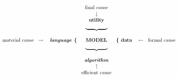
While the linear view expresses the creation of a model as a linear sequence of operations, the developmental view interprets the model as resulting from the interaction of four restraints acting upon it. These restraints can be formalized with the scheme in Figure 2. The model to be learned is constrained between four surrounding layers in an intersecting specification hierarchy (Salthe, 1993). Under these restraints, the model emerges organically. The restraints need not be fixed. On the scalar scale, the modelling is performed inside the agent.
Utility, language, algorithm and data can be interpreted as Aristotelian causes of the model: the model cannot be independent of either of them. The algorithm is what is driving the construction of the model. The language is what the model is made of. The data is what defines the form of the model: obviously the model should be consistent with the empirical data. Finally, the model is going to be judged though the utility of the actions chosen by using the model.
 Figure
2: The model develops under the pressure of constraints. The constraints
are the Aristotelian causes: the capacity of the algorithm, the expressive
power of the language, the quest for utility and the consistency with the data.
Figure
2: The model develops under the pressure of constraints. The constraints
are the Aristotelian causes: the capacity of the algorithm, the expressive
power of the language, the quest for utility and the consistency with the data.
3. Dichotomies in Learning
There are numerous views of inductive learning and statistical inference. Machine learning is still an active field of research and there are different methodologies competing with one another. With a bit of emotional distance we see, however, that many of the competing approaches in fact approach the same problem, but from a different direction. Our description will briefly and simply touch upon several ideas in machine learning, artificial intelligence and statistics. The list should be seen as an opinionated snapshot, not as an exhaustive survey.
3.1. Identification vs Approximation
The Probably Approximately Correct (PAC) learning theory (Valiant, 1984) was concerned with problems of deductive identification. We assume that the data results from measurement of a specific but unknown concept that determines whether an instance is true or not. The concept itself is a statement in a particular language, and the task of learning is to identify the concept that yielded the instances. Valiant proved that the learning problem is tractable for several non-trivial concept languages, such as conjunctive and disjunctive normal form expressions. The criterion in this identification approach is to arrive at the true definition of the concept. Here, our term `identification' is to be distinguished from `system identification', an approach to modelling which includes approximation.
The utility is not needed because the language is trusted. The language is the ontology. Most scientists believe that mathematics is the right language for modelling nature, for example. We often like to think that our brain (as a kind of a language) is powerful enough to understand the truth of the universe. Many philosophers deem that the language of causal logic is sufficient for a complete description of how the universe evolves and revolves, and that everything can indeed be linked into an endless thread of chain and effect.
Identification assumes that the agent's language
matches the language of the concept. This is a strong assumption: we are rarely
sure that our language as such can truly describe the reality! For that reason,
the agnostic approach to learning (Haussler,
1992) no longer expects that the model will be true. The approximation
approach no longer seeks truth, but only seeks to minimize the error that the
model makes. The language is epistemology. For example, the agent will decide between
using the barometer, the weather channel, or a combination of both in order to
minimize the error in predicting the weather next day. The goal is achieved
when the agent finds the best of the models that can be expressed with its
language. This way, however, trust is placed onto utility as a realistic model
of model quality. For example, we may assume the utility to be the mean square
error:
1/nåi = 1n(yi - y(xi))2, for n test
instances áy1,x1ñ ,...,áyn,xnñ that have the true value of yi, which can be
predicted from xi
as y(xi).
While the identification approach strives to explain the nature with a specific language, reducing data into special cases of particular universal truths, the approximation approach is sceptical about the validity of the language. Of course, a good enough model can be found in the language, but perhaps there is another language that would work even better. An old joke says: The approximating engineer thinks that equations approximate the reality, while the identifying physicist thinks that the reality approximates the equations.
3.2. Probability: Frequency vs Belief
In many circumstances it is impossible to predict the outcomes exactly. I take a coin and toss it, but even if I try, I cannot perfectly control the outcome. If it is not possible to reliably predict the outcome, we can still reliably predict the probability of each outcome. For example, we could say that there is a 50% probability of the coin falling heads, and a 50% probability of the coin falling tails.
There are numerous interpretations of the meaning of probability, but a particularly important division is into the frequentist probability on one hand and the interpretation of probability as a degree of belief on the other hand. Objective frequentist probabilities are a part of the ontology, and they refer to reality. On the other hand, subjective beliefs arise from agent's limited knowledge about the world, and are an aspect of epistemology. The worldview with frequentist probability takes the reality as inherently unpredictable, but guided by a true model. The true model is identifiable, should an infinite number of observations be made. Probability is defined through the long-run frequency of an event. Learning is referred to as estimation, and seeks to minimize the fixed utility or risk.
On the other hand, the subjective view considers probabilities as resulting from the lack of knowledge. The coin toss, for example, appears random purely because the conditions of each experiment are not precisely controlled. Learning is referred to as inference. The probability is thus seen just as a way of representing the degree of belief, the ignorance, the inability or reluctance to state a deterministic model. The subjective probability refers to statements in a language, not to objects in the world. It is the model that is unable to predict the outcome, perhaps due to agent's bad eyes or thick fingers, not the inherent unpredictability of the reality. An ideal observer with all the information would be able to get a model with less uncertainty. A subjective interpretation of an unpredictable quantum phenomenon is that we do not know what is inside, not that the inside is inherently unknowable. The process of learning seeks to maximize the utility of the model, but the utility and the probability are dependent and inherently entangled (Rubin, 1987). It is possible, however, to use proper score functions and objective algorithms that favor probabilities that are calibrated and have good properties with respect to the frequentist criteria.
3.3. Simplicity vs Timidity
The simplicity-driven algorithm restricts itself to a simple language and then seeks the best model from the language, in the process of fitting or optimization. It is a good practice to assess whether the model is significantly better than another simpler model. It is also possible to reverse the process: we first identify the best model, and then seek to simplify it in the process of pruning (Breiman et al., 1984). In all, simplicity-driven algorithms restrict the language or hide the data, and then maximize the performance.
The grand majority of scientists pursue simplicity. Namely, the goal of learning is not just to predict but also to understand. A simple explanatory model of a previously complicated phenomenon is the epitome of science. When the model appears too complex, it is critiqued and disliked: the simplicity has an inherent quality to it, a quality that does not derive from the objective precision of the model. Instead, simplicity implies that the model is easier to learn, keep in mind, work with, easier to present on a slide, easier to persuade people into it, and easier to validate.
On the other hand, the timidity-driven approach tries to identify the model that agrees with the data but that achieves the highest utility in the worst case. For example, we examine the data and estimate particular statistics, such as the mean and the standard deviation. Now, what model with such a mean and such a standard deviation is the most timid in the sense that it will be worst-case optimal according to some utility function? The most timid one is the bell-curved Gaussian distribution. If our constraints are the upper and the lower limit, the most timid model is the uniform distribution. Generally, the constraints imposed upon the model ascertain that the model agrees with the data. But from all agreeable models, we pick the least pretentious one of them, which also has the property of worst-case optimality. Generalizations of this view are the maximum entropy (MaxEnt) methods (Jaynes, 2003). Another interpretation is that the maximum entropy model is the most `settled-down' model that the constraints allow, a view that resonates well with the organic view of Figure 2.
3.4. Selection vs Combination
There may be multiple models within a single language that are all consistent with the data. The set of consistent models is referred to as the version space (Mitchell, 1997). There are two approaches for resolving this issue: model selection and model combination. Model selection seeks to identify the single best model. Model combination instead views the identity of the model as a nuisance parameter: no model is correct, but we can assign each model a weight accordant with its performance. It must be stressed that we are not selecting actions. Instead, we are selecting models, and the selected model will be used to select actions.
There are very many model selection criteria. For example, Fisher's maximum likelihood principle (Fisher, 1912) suggests picking the single most likely model, regardless of anything else. Hypothesis testing in statistics selects a particular null model unless there is overwhelming evidence against it. The Bayesian priors (Bernardo & Smith, 2000) set up a coherent set of preferences among models that are combined with the models' likelihoods. Ockham's parsimony principle prefers the simplest among several equally useful models. The maximum entropy approach (Jaynes, 2003) prefers the `flattest' and most symmetric model with the highest Shannon entropy of all those that satisfy the constraints derived from the data. Akaike information criterion (AIC) (Akaike, 1973) penalizes the utility with the number of parameters. The minimum description length principle (Rissanen, 1986) represents the complexity of the model with the same unit of measurement as the utility.
An example of the application of model selection is shown in Table 3. There are four models: NBC, PIG, NIG and BS. These four models are applied to several data sets, and the one that achieved the lowest loss (loss is the opposite of utility) is typeset in bold. It can be seen that the model NBC very often achieves the best performance. Only in a few situations BS performs better. Overall, however, NBC would be selected as `the best'.
|
|
NBC |
PIG |
NIG |
BS |
|
lung |
0.230 |
0.208 |
0.247 |
0.243 |
|
soy-small |
0.016 |
0.016 |
0.016 |
0.016 |
|
zoo |
0.018 |
0.019 |
0.018 |
0.018 |
|
lymph |
0.079 |
0.094 |
0.077 |
0.075 |
|
wine |
0.010 |
0.010 |
0.015 |
0.014 |
|
glass |
0.070 |
0.071 |
0.071 |
0.073 |
|
breast |
0.212 |
0.242 |
0.212 |
0.221 |
|
ecoli |
0.032 |
0.033 |
0.039 |
0.046 |
|
horse-c |
0.108 |
0.127 |
0.106 |
0.104 |
|
voting |
0.089 |
0.098 |
0.089 |
0.063 |
|
monk3 |
0.042 |
0.027 |
0.042 |
0.027 |
|
monk1 |
0.175 |
0.012 |
0.176 |
0.012 |
|
monk2 |
0.226 |
0.223 |
0.224 |
0.226 |
Table 3: Model selection. The losses (negative utilities) suffered by different modelling methods (NBC, PIG, NIG, BS) are not consistent across data sets. For each row we can select the one of the best methods, typeset in bold, for that particular data set. It is difficult, however, to choose a single best method overall.
Sometimes, however, the choice is ambiguous: the problem is illustrated in Figure 3: two models A and B were tested over a large number of experiments in two contexts. For each experiment, the utility of model B was subtracted from the utility of model A.
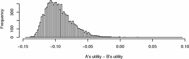
Figure 3: Replicated comparisons. We can compare the utility of two models over several experiments. Sometimes it is easy (top), and sometimes hard (bottom) to decide which model is better, A or B.
In the first case (top), the model B achieved higher utility than model A almost always. However, in a small number of situations A was better. In the second case (bottom), deciding which model is better becomes a very difficult problem: in the most frequent case (mode), B was better; for the average utility over all experiments, A was better; in the average case (median), B was better; in the best case, A was better; at the worst, B was not as bad. What to do? Deciding between two models may be ambiguous even when the consistent and quantitative utilities are given in full detail. Of course, such a dilemma only arises when the methods are similar in performance, and any choice might be fine.
Epicurus' principle of indifference states (Kirchherr et al., 1997): Keep all hypotheses that are consistent with the facts. Therefore, instead of making an arbitrary selection, one could perform a combination. Consistency is not a binary decision: in a probabilistic context several models have a non-zero posterior probability, meaning that they are all consistent, to some extent. Namely, if we see three tornadoes in the same week, it might be due to the expected pattern with global warming or simply due to a coincidence without global warming. The Bayesian solution to this problem is based upon an ensemble of multiple models, with each model having non-zero likelihood. In our example, we would consider both global warming and no global warming as being true to some extent. The term commonly used for the ensemble is the posterior distribution over the models, but the whole ensemble itself is really a single model, composed of submodels.
Let us consider the familiar example of the coin toss. There are numerous languages that can formalize our knowledge about the coin. One language views the coin as guided by some frequentist probability: the greater the probability of the coin falling heads, the larger the frequency of the heads in the final tally. A model from this language is referred to as the Bernoulli model. We start with some prior belief about the coin's probability: the coin may be biased, or unbiased.
|
|

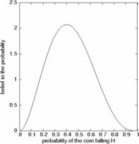
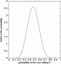
Figure 4: A Bayesian ensemble of models. Each probability of the unknown coin falling heads is an individual submodel, and these submodels form an ensemble. Each submodel is assigned a particular belief. Our prior belief is uniform over all the probabilities. Successive observations of coin toss outcomes induce greater and greater precision in our beliefs about the posterior probability (left to right). Still, there is always some uncertainty about the exact probability.
We can represent this belief by saying that our prior is an ensemble of all possible Bernoulli submodels, and our belief in each submodel is equal (Figure 4, left panel). Then we toss the coin five times, and the tally is 3 tails and 2 heads. The resulting ensemble reflects this (Figure 4, middle panel): those probabilities that indicate that the coin always falls heads are impossible, and the most likely is the submodel that claims that the probability of heads is 2/5. The data has narrowed the range of our beliefs about the probability. It would be improper, however, to claim that this single submodel is representative of the coin: we have not seen enough data to be so specific. All we can say is that we believe that the probability of heads is in the interval [0.1,0.8]. Performing a few more tosses, we end up with the tally of 9 heads and 10 tails. The distribution of our beliefs over the ensemble ( Figure 4, right panel) shows that the probability is almost certainly somewhere on [0.2,0.8], but we cannot yet say anything beyond that with complete certainty.
When such an ensemble is used to make a prediction, each submodel makes a distinct prediction. This way, we obtain an ensemble of predictions, each of them weighted by the posterior probability of the corresponding submodel. We can interpret the ensemble as an imprecise prediction: not just that the ensemble is not sure about the outcome, it is also unsure about the probability. The other way of interpreting the ensemble is by stating that the true submodel is a nuisance parameter, a property that exists but we do not want to know. The Bayesian approach for dealing with nuisance parameters is to average the predictions of all submodels, so that each prediction is weighted by our belief in the submodel that made it.
If we consider the submodel as a nuisance parameter, we need not treat the model as an ensemble: it is somewhat expensive to lug along all the submodels and their individual worths. Instead, we may average them together. In this case, we can represent the average as a single model being guided by the following probability:
![]()
This is referred to as the Laplace estimate of probability, because the legend says that Laplace wondered about the probability of seeing another sunrise after having seen only a single one.
Of course, in some applications it is important to keep note of the whole ensemble: pMAPH is identical for the tally of 1 head and 1 tails and for the tally of 10000 heads and 10000 tails. However, the ensemble is much more distinctly peaked for the latter one. Averaging, therefore, is a way of replacing the Epicurean ensemble with a single submodel that is closest to the average of the ensemble, but any single submodel from the ensemble does not faithfully represent the variation in the ensemble. There is an old statistician's joke: The average European has one testicle and one ovary.
3.5. Bias vs Variance
Would you believe me if I told you that all ravens are black after seeing five of them? In every case, the agent is restricted to the data set. The agent seeks the elusive goal of generalization (Wolpert, 1995): the model should be applicable to data that has not been used when building the model, the model should be the best on the data that was not yet seen. This problem is highly problematic: what can we know about the data we have not seen?
The cross-validation approach (Stone, 1974) divides the data into two parts: one part is used for building the model, and the second part for evaluating its utility; this way we prevent the model from simply memorizing the instances and `peeking at the correct answers'. We are interested in the agent generalizing, not memorizing. Thus, we evaluate the agent's predictions on those instances that it has not seen during learning of the model. This way, the validated utility will reflect the mistakes of generalization. The idea underlying the cross-validation is that a reliable model will be able to show a consistent gain in utility with incomplete data. By induction, we then expect that a model that achieved reliable performance with a part of the given data will also not miss the target on the future truly unseen data.
The hidden nuisance parameter in cross-validation is how much data we use for training. This decision is far from arbitrary, as we will now show using learning curves (Kadie, 1995). A learning curve shows the relationship between the performance of a model on unseen data depending on how much data was used for training. If the utility no longer changes, the model has converged, and additional data is less likely to affect the model.
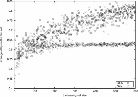
Figure 5: The learning curves. Most models become better with an increasing number of instances. Some of them quickly reach a plateau and result in reliable utility. Others take more chances, and reach greater levels of utility, but pay a cost in reliability.
In Figure 5 we compare two commonly used algorithms in machine learning, the naive Bayesian classifier (NBC), and the C4.5 classifier (Quinlan, 1993). The utility is not simple to characterize when there is little data (less than 50 instances), but NBC is less robust than C4.5. When there is more data (50-150), it is still difficult to compare both methods. Beyond 150 instances, NBC becomes reliable: we know that the NBC model requires approximately 150 instances to be characterized almost unambiguously. On the other hand, C4.5 keeps gaining utility indefinitely. Therefore, two conclusions can be made: the NBC model is simple enough to be identified unambiguously from 300 instances; this is a good result, as there are 960 instances in that data set. And, when there are 250 instances, the C4.5 model has not yet fully converged, but it is already clear that it is consistently better than the NBC model.
Still, there is the problem of which method to choose: C4.5 has higher average utility, but NBC has lower variance in its utility. This trade off is referred to as the bias/variance dilemma (Geman et al., 1992). When we want to be sure about the performance, in cases when any mistake would be dangerous, a method with lower variance is preferable. When, however, we can afford to take chances, the method with lower bias is going to be preferable, in spite of the possible variance. The choice of the model, hence, depends on how risk-averse we are. It is clear, though, that the generalization performance still depends on the sample being unbiased representative: when one wants to predict the outcome of the elections, one should ask the people that will actually vote, and even these should not be all aging golf players but instead a representative sample of the whole population (that will vote). No cross-validation on the population of aging golf players will reveal the true preferences of the general population. Also, problems occur both with learning curves and cross validation when there are very few instances: then neither the convergence nor the average utility can be reliably assessed.
There is an important connection between simplicity and variance. It is often thought that simple models have lower variance, but it would be mistaken to assume that this connection is causal or rigid. Whether a complex language will yield models with high variance depends upon the prior assumptions and on the algorithm. Seemingly complex models often have low variance (Breiman, 1996).
3.6. Bayesians vs Frequentists
A common dilemma in statistics is between the opponents and endorsers of the Bayesian approach. We will now present their caricatures. For a frequentist, there are multiple data sets consistent with a given model: their probabilities are about the data, and their model is believed to be true. For a Bayesian, there are many models in the language that are consistent with a particular piece of data: each model has a specific belief, but their data is assumed to have the probability of 1.
Bayesians are uncertain about the model, but assume certainty about the data. To get rid of the uncertainty, they average out the model. To demonstrate the uncertainty, they perturb the choice of the model given a data set, and examine if the ensemble can be faithfully represented by a model selection or a model average. Bayesians tend to be driven by languages and data: they focus on the construction of languages to model data. Their priors are the explicit gold standard, and the algorithms they use are centered on the properties of the priors and the data. In fact, with the scheme of Figure 2, their algorithm is really the prior.
Frequentists are uncertain about the data, but assume certainty about the model. To demonstrate the uncertainty, they perturb the data given a model. To get rid of the uncertainty about the model, they vary the data, and select the best model of a particular language for the data. For different choices and sizes of the data, they compare the languages on the bias-variance axis. If the variance is too high, they average over the selections. Frequentists tend to be driven by utilities and algorithms: they focus on the construction of algorithms to maximize utilities. They rarely question their language (which is usually very flexible), and their prior assumptions are hidden in the choice of the algorithms.
Because the assumptions are different, attempts to reconcile these approaches are difficult. Frequentists find it illogical that a photon detector would have `beliefs' about the outcomes. Bayesians would respond that there may be laws in the nature, but all we can do is to have beliefs about them. On the other hand, Bayesians find it illogical for a frequentist to say that there is a probability in the world that rules the outcome of a coin toss. Frequentists would respond that the probability would arise if such experiment was repeated in identical circumstances infinitely many times, or through Everett's many-worlds interpretation of probability (Everett, 1957).
To be fair, most frequentists in statistics do not think in such a way: most statisticians tend to be epistemological in spirit, and true frequentists may be found among the ontologically-minded physicists. The statisticians that do not call themselves frequentists but non-Bayesians pragmatically prefer to work with the algorithms and the utilities, rather than to work indirectly through languages, like Bayesians. And most Bayesians too are pragmatic and concerned about various utility functions and algorithms. Still, there are attempts to reconcile the results if not their interpretations (Berger, 2003). It is important, however, to see that beliefs and probabilities can co-exist.
4. Subjective, Intersubjective and Objective
There is also the dilemma of identification and approximation. It is clear that once the ontology is fixed, and if the ontology includes probability, frequentist probability is an existent which we can seek to estimate. But if the ontology is internal and not external, one has to include epistemological considerations with prior expectations and degrees of belief. The opponents of this approach argue that the choice of the prior is inherently subjective. The Bayesians struggle to find `objective' languages and prior assumptions, ones that carry little bias or preference for different models. An example of such priors are the non-informative priors, ones that provide no information about the choice of the model and reflect ignorance. It is easy to dismiss these attempts as `still subjective'.
The most common example of an `objective' technique is the linear regression model. It is next to being fully automated: no human intervention is needed beyond preparing reliable, plentiful and unbiased data. It has been used for numerous applications, often resulting in utility. It is widely accepted and known. It is taught in schools. Many people understand linear models and can gain utility from them. But this does not make linear regression objective. It is just a specific model, based upon many subjective assumptions. The very fact that we are assuming that a linear model can be used to represent reality is quite arbitrary. Nobody really believes that the nature is solving linear equations.
The key difference, thereby, is that `objective' methods result in models that are transplantable, multisubjective or intersubjective. Intersubjective models are self-sufficient and encapsulated, they are particulars. This way, they can be communicated from one agent to another. Furthermore, transplantable models derive from shared preconceptions; they are guided by rules that are general. They do not make use of the hidden implicit subjective assumptions, but only of those prior assumptions that are shared by several agents. In summary, intersubjectivity means that a model can be understood and accepted by more than a single agent in a community. But intersubjective approaches are still epistemological, so ontologists do not find them objective.
It is not just that shared language (otherwise a model could not be conveyed), shared data (otherwise the model could not be verified), and shared algorithms (other the model could not be proved) that matter: shared utilities matter too. Someone might understand my theory, but the question is whether the other agent will appreciate it as much as I do. I might form an intersubjective and comprehensible theory of why there are five empty cups of coffee on my desk, but not many agents will care: my model of the five cups does not yield them any utility. In all, objective models arise from data, algorithms, utilities and languages that are shared by the whole community. Sometimes, we convey them explicitly (“Tomorrow is going to rain.”), and sometimes by conveying merely their causes (new data, new rules of induction, new words in the language, new qualities and priorities).
The four Aristotelian causes (data, algorithms, language, and utility) must be aligned for the model to coalesce. Teaching is about varying one or two of the causes so that the learner can re-adjust his internal model. If too many causes are varied, if there is no alignment, or if there is imbalance along any of the dichotomies listed in the previous sections, the learner becomes confused and lost. Therefore, it is desirable for only one of the causes to be varied during teaching. Communicating the data is the easiest of all causes. It may even turn out that the data is the only way of conveying models: A theory is something nobody believes, except the person who made it. An experiment is something everybody believes, except the person who made it.
ACKNOWLEDGEMENTS
The author has benefitted from and was influenced by discussions with S. Salthe, M. Forster, J. McCrone, C. Lofting and E. Taborsky.
REFERENCES
Akaike, H. 1973. Information theory and the maximum likelihood principle. In Petrov, B. N. & Csaki, F. (Eds.), Second International Symposium on Information Theory. Budapest: Akademiai Kiado.
Berger, J. 2003. Could Fisher, Jeffreys and Neyman have agreed upon testing? Statistical Science, 18, 1–32.
Bernardo, J. M. & Smith, A. F. M. 2000. Bayesian Theory. Chichester: Wiley.
Breiman, L. 1996. Bagging predictors. Machine Learning, 24(2), 123–140.
Breiman, L., Friedman, J. H., Olshen, R. A. & Stone, C. I. 1984. Classification and Regression Trees. Belmont, CA: Wadsworth.
Everett, H. 1957. Relative state formulation of quantum mechanics. Reviews of Modern Physics, 29, 454–462.
Fisher, R. A. 1912. On an absolute criterion for fitting frequency curves. Messenger of Mathematics, 41, 155–160.
Geman, S., Bienenstock, E. & Doursat, R. 1992. Neural networks and the bias/variance dilemma. Neural Computation, 4, 1–58.
Haussler, D. 1992. Decision theoretic generalizations of the PAC model for neural net and other learning applications. Information and Computation, 100(1), 78–150.
Jaynes, E. T. 2003. In G. L. Bretthorst (Ed.), Probability Theory: The Logic of Science. Cambridge, UK: Cambridge University Press.
Kadie, C. M. 1995. Seer: Maximum Likelihood Regression for Learning-Speed Curves. PhD thesis, University of Illinois at Urbana-Champaign.
Kirchherr, W., Li, M. & Vitányi, P. M. B. 1997. The miraculous universal distribution. Mathematical Intelligencer, 19(4), 7–15.
Mitchell, T. M. 1997. Machine Learning. New York, USA: McGraw-Hill.
Quinlan, J. R. 1993. C4.5: programs for machine learning. San Francisco, CA: Morgan Kaufmann Publishers Inc.
Rissanen, J. 1986. Stochastic complexity and modeling. Annals of Statistics, 14, 1080–1100.
Rubin, H. 1987. A weak system of axioms for `rational' behaviour and the non-separability of utility from prior. Statistics and Decisions, 5, 47–58.
Russell, S. J. & Norvig, P. 1995. Artificial Intelligence: A Modern Approach. New Jersey, USA: Prentice-Hall.
Salthe, S. N. 1993. Development and Evolution: Complexity and Change in Biology. MIT Press.
———, 2001. Theoretical biology as an anticipatory text: The relevance of Uexküll to current issues in evolutionary systems. Semiotica, 134(1/4), 359–380.
Stone, M. 1974. Cross-validatory choice and assessment of statistical predictions. Journal of the Royal Statistical Society B, 36, 111–147.
Valiant, L. 1984. A theory of the learnable. Communications of the ACM, 27(11), 1134–1142.
Wolpert, D. H. (Ed.). 1995. The Mathematics of Generalization, Proceedings of the SFI/CNLS Workshop on Formal Approaches to Supervised Learning, Santa Fe Institute. Addison-Wesley.